tourrr: Exploring multi-dimensional data

R
TIL
Author

Thomas Sandmann

Published

August 28, 2023

tl;dr

Today I learned about exploring multivariate data using tours of projections into lower dimensions. The tourr R package makes it easy to experiment with different tours. Let’s go on a grand tour!

Introduction

Earlier this month, Dianne Cook and Ursula Laa published Interactively exploring high-dimensional data and models in R, a free online book accompanied by the mulgar R package. It’s a great introduction to exploratory analysis of multivariate data πŸš€.

The authors introduce data tours to interactively visualize high-dimensional data. (And also highlight the rich history of this field, including the PRIM-9 system created at Stanford in the early 1970s ).

The tourr R package provides user-friendly functions to run a tour.

A gorilla hiding in plain sight

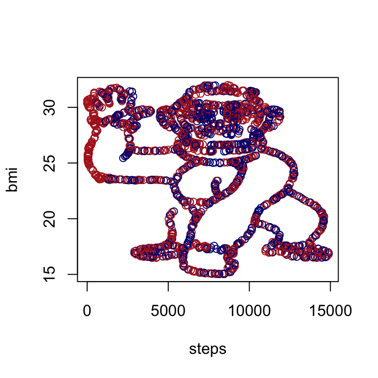
In 2020, Itai Yanai and Martin Lercher asked whether β€œfocus on a specific hypothesis prevents the exploration of other aspects of the data”. 1 They simulated a dataset with two variables, bmi and steps for both male and female subjects. Let’s start with a similar dataset 2.

gorilla <- read.csv(
  paste0("https://gist.githubusercontent.com/tomsing1/",
         "d29496382e8b8f4163c34df46b00686f/raw/",
         "40c0b7b5d25fff188a7365df59aa8634fef9adb9/gorilla.csv")
)
with(gorilla, plot(steps, bmi, col = ifelse(group == "M", "navy", "firebrick")))

Here, we want to examine only the numerical measurements (e.g. bmi and steps ), so let’s remove the categorical group variable and add two noise variables to create a dataset with five numerical variables.

for (dimension in paste0("noise", 1:2)) {
  gorilla[[dimension]] <- rnorm(n = nrow(gorilla))
}
numeric_cols <- setdiff(colnames(gorilla), "group")
head(gorilla)
       bmi      steps group     noise1     noise2
1 29.96000   145.6311     F  0.2262401 -0.2269717
2 29.89818 10048.5437     M -1.0365464 -0.9440436
3 23.46909  3859.2233     M  0.5676465 -0.6378377
4 26.03455  7718.4466     M -2.3049200 -0.5047930
5 19.51273 10776.6990     M  0.4935926 -0.5288485
6 29.65091  3932.0388     M  1.0021255 -1.1318410

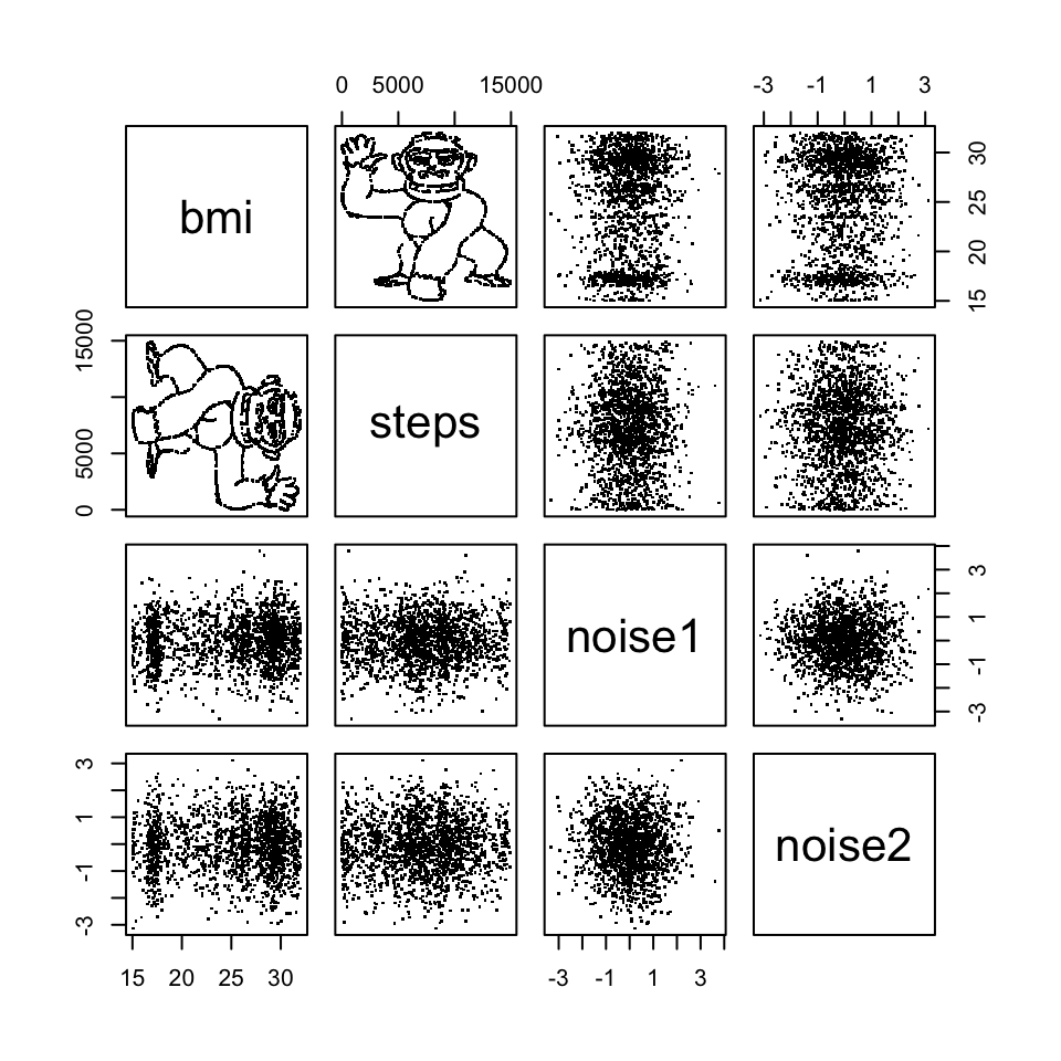
Plotting all pairwise combinations of the 5 variables quickly reveals the gorilla hidden in the bmi ~ steps relationship:

pairs(gorilla[, numeric_cols], pch = ".")

Taking tours

library(tourr)
library(gifski)  # to create animated gifs
gorilla[, numeric_cols] <- tourr::rescale(gorilla[, numeric_cols])
clrs <- c("#486030", "#c03018", "#f0a800")
group_col <- clrs[as.numeric(factor(gorilla$group))]

Taking a little tour

The little tour cycles through all axis parallel projections, reproducing all of the static plots we obtained with the pairs() call above (corresponding to 90 degree angles between the axes) as well as additional projections in between.

As expected, the gorilla cartoon reveals itself whenever the steps and bmi variables are projected into the x and y coordinates.

if (interactive()) {
  tourr::animate(data = gorilla[, numeric_cols], 
                 tour_path = little_tour(d = 2), 
                 display = display_xy())
} else {
  tourr::render_gif(
    data = gorilla[, numeric_cols],
    little_tour(), 
    display_xy(),
    gif_file = "little_tour.gif",
    width = 300,
    height = 300,
    frames = 500,
    loop = TRUE
  )
}

Little tour

Grand tour

The grand tour picks a new projection at random and smoothly interpolates between them, eventually showing every possible projection of the data into the selected number of dimensions (here: 2). With a very high dimensional dataset, traversing all possibilities can take quite a while.

if (interactive()) {
  tourr::animate(data = gorilla[, numeric_cols], 
                 tour_path = grand_tour(d = 2), 
                 display = display_xy())
} else {
  tourr::render_gif(
    data = gorilla[, numeric_cols],
    grand_tour(d = 2), 
    display_xy(),
    gif_file = "grand_tour.gif",
    width = 300,
    height = 300,
    frames = 500,
    loop = TRUE
  )
}

Grand tour

Adding interactivity

Dianne Cook’s and Ursula Laa’s book also demonstrates how to make the tours more interactive with the plotly and htmlwidgets R packages.

Code to generate interactive animation
library(plotly, quietly = TRUE)
library(htmlwidgets, quietly = TRUE)
set.seed(123)
subsample <- sample(nrow(gorilla), size = 500L)
pn_t <- tourr::save_history(data = gorilla[subsample, numeric_cols], 
                            tour_path = grand_tour())
pn_t <- interpolate(pn_t, angle = 1)
pn_anim <- render_anim(gorilla[subsample, numeric_cols], frames = pn_t)

pn_gp <- suppressWarnings({
  ggplot() +
    geom_path(
      data = pn_anim$circle, 
      aes(x = c1, y = c2, frame = frame - 100), 
      linewidth = 0.1) +
    geom_segment(
      data = pn_anim$axes, 
      aes(x = x1, y = y1, xend = x2, yend = y2, frame = frame - 100), 
      linewidth = 0.1) +
    geom_text(
      data = pn_anim$axes, 
      aes(x = x2, y = y2, label = axis_labels, frame = frame - 100), 
      size = 5) +
    geom_point(
      data = pn_anim$frames, 
      aes(x = P1, y = P2, frame = frame - 100), 
      alpha = 0.8, size = 0.5) +
    xlim(-0.8, 0.8) + ylim(-0.8, 0.8) +
    coord_equal() +
    theme_bw() +
    theme(axis.text = element_blank(),
          axis.title = element_blank(),
          axis.ticks = element_blank(),
          panel.grid = element_blank())
})
ggplotly(
  pn_gp,
  width = 500,
  height = 550) %>%
  animation_button(label="Go") %>%
  animation_slider(len = 0.8, x = 0.5, xanchor = "center", 
                   currentvalue = list(prefix = "frame: ")) %>%
  animation_opts(easing = "linear", transition = 0)

Reproducibility

Session Information
sessioninfo::session_info("attached")
─ Session info ───────────────────────────────────────────────────────────────
 setting  value
 version  R version 4.3.1 (2023-06-16)
 os       macOS Ventura 13.5.1
 system   aarch64, darwin20
 ui       X11
 language (EN)
 collate  en_US.UTF-8
 ctype    en_US.UTF-8
 tz       America/Los_Angeles
 date     2023-08-30
 pandoc   3.1.1 @ /Applications/RStudio.app/Contents/Resources/app/quarto/bin/tools/ (via rmarkdown)

─ Packages ───────────────────────────────────────────────────────────────────
 ! package     * version  date (UTC) lib source
 P ggplot2     * 3.4.3    2023-08-14 [?] CRAN (R 4.3.0)
 P gifski      * 1.12.0-2 2023-08-12 [?] CRAN (R 4.3.0)
 P htmlwidgets * 1.6.2    2023-03-17 [?] CRAN (R 4.3.0)
 P plotly      * 4.10.2   2023-06-03 [?] CRAN (R 4.3.0)
 P tourr       * 1.1.0    2023-08-24 [?] CRAN (R 4.3.0)

 [1] /Users/sandmann/repositories/blog/renv/library/R-4.3/aarch64-apple-darwin20
 [2] /Users/sandmann/Library/Caches/org.R-project.R/R/renv/sandbox/R-4.3/aarch64-apple-darwin20/ac5c2659

 P ── Loaded and on-disk path mismatch.

──────────────────────────────────────────────────────────────────────────────

Creative Commons License
This work is licensed under a Creative Commons Attribution 4.0 International License.

Footnotes

  1. In addition to being asked what they could conclude from the dataset, half of the students were asked to also test specific hypotheses. […] students in the hypothesis-free group were almost 5 times more likely to observe an image of a gorilla when simply plotting the data, a proxy for an initial step towards data analysis.β†©οΈŽ

  2. Matt Dray showed how to recreate the dataset using R in this great blog post., the code to generate the gorilla dataset I use here is in this gist.β†©οΈŽ